Statistical Mechanics
Thermodynamics gives us the laws of macroscopic systems. Mechanics gives us the laws of microscopic particles. Statistical Mechanics is the rigorous mathematical bridge that unites them.
1. Phase Space & The Ergodic Hypothesis
Imagine a box of gas containing molecules. If we wanted to solve this system using classical Newtonian mechanics, we would need to write down coupled differential equations for every single particle. Even if a supercomputer could track this, the resulting data—trillions of trajectories—would be utterly useless to us. We don't care about the trajectory of molecule #4,000,000. We care about macroscopic observables: pressure, temperature, and volume.
To begin, we define the microscopic state of the entire system as a single point in a -dimensional manifold called Phase Space (). This space is spanned by generalized coordinates and conjugate momenta .
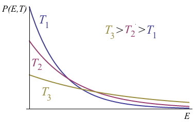
Fig 1: A point representing the entire system traces a trajectory through Phase Space. By Liouville's Theorem, a local volume of these points evolves like an incompressible fluid.
As time ticks forward, the system evolves according to Hamilton's equations, and this point traces a trajectory through phase space. Instead of tracking a single system, Josiah Willard Gibbs introduced the concept of an Ensemble—an infinite collection of mental copies of our system, all in different microstates but sharing the same macroscopic constraints.
The foundation of this framework relies on the Ergodic Hypothesis. It states that over a long period of time, the time spent by a system in some region of phase space of microstates with the same energy is proportional to the volume of this region. Simply put: Time averages equal ensemble averages.
2. The Microcanonical Ensemble (Isolated Systems)
Let us start with the simplest possible scenario: a completely isolated system. It cannot exchange energy (), volume (), or particles () with its surroundings. This is the Microcanonical Ensemble.
In this isolated state, the system is governed by a singular, breathtakingly bold axiom known as the Fundamental Postulate of Statistical Mechanics:
"In an isolated system in thermal equilibrium, every accessible microstate is equally probable."
Nature does not play favorites. If a microstate possesses the correct total energy , the system is just as likely to be found in that state as any other. Let denote the total number of accessible microstates. The probability of finding the system in any specific microstate is simply .
Ludwig Boltzmann realized that this combinatorial counting was directly related to the macroscopic concept of entropy. His legendary formula, famously engraved on his tombstone in Vienna, is:
Boltzmann's Entropy
This equation fundamentally demystifies entropy. It is not some invisible thermodynamic fluid; it is simply a logarithmic measure of our ignorance. From this single equation, the entirety of thermodynamics can be derived. For example, temperature is defined geometrically as the slope of entropy with respect to energy:
Statistical Definition of Temperature
3. The Canonical Ensemble (Fixed Temperature)
Isolated systems are mathematically beautiful, but experimentally rare. Real systems exchange heat with their environment. Imagine placing our small system in contact with an infinitely large thermal reservoir at a fixed temperature . They can exchange energy, but the total energy remains constant. This is the Canonical Ensemble.
Because the reservoir is so massive, if our system adopts a microstate with a very high energy , it robs the reservoir of that energy. The reservoir's entropy plummets, making this configuration highly statistically unlikely. Through a Taylor expansion of the reservoir's entropy, we find that the probability of our system being in state decays exponentially with energy. This is the Boltzmann Distribution:
The Boltzmann Factor
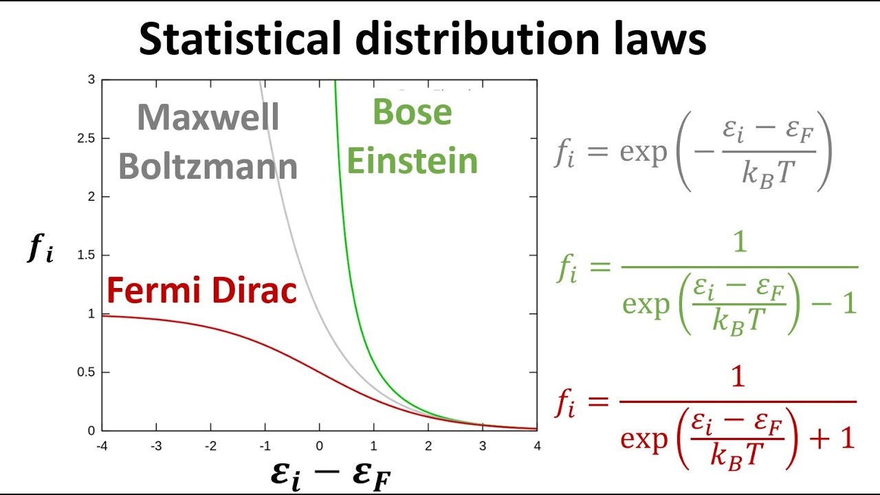
Fig 2: The exponential decay of microstate probability. Notice how at higher temperatures (lower beta), the distribution flattens, allowing the system to access higher energy states more frequently.
The normalization constant is arguably the most important quantity in all of physics. It is the Partition Function (from the German Zustandssumme, meaning "sum over states").
The Canonical Partition Function
As Richard Feynman taught, "If you know the partition function, you know everything." It acts as a generating function for the thermodynamics of the system. By taking the logarithm of , we directly recover the Helmholtz Free Energy :
Helmholtz Free Energy
Once you have , macroscopic observables are just derivatives. Pressure is . Entropy is . Average energy is . The entire physics of the system is compressed into the algebraic form of .
4. The Grand Canonical Ensemble (Variable Particles)
What if the system is open? What if it can exchange both heat and particles with the reservoir? This is the Grand Canonical Ensemble. The system is now defined by its volume , temperature , and Chemical Potential .
The chemical potential acts as the "cost" of adding a particle to the system. The probability of the system having exactly particles and being in microstate becomes:
Gibbs Factor
Here, is the Grand Partition Function. This ensemble might seem like a mathematical overcomplication, but it is an absolute necessity when dealing with quantum gases, where the number of particles in a specific quantum energy level is constantly fluctuating.
5. The Ideal Gas & Gibbs Paradox
Let's apply this machinery to a classical ideal gas: non-interacting point particles in a box. Because they don't interact, the total energy is just the sum of their individual kinetic energies: .
When we calculate the partition function by integrating over phase space, something bizarre happens. If we calculate the entropy, we find that it doesn't scale linearly with the size of the system. If we mix two identical boxes of identical gas, the math says the entropy increases—even though nothing physically changed! This is the Gibbs Paradox.
The resolution to this paradox required a radical, pre-quantum realization: Particles of the same species are fundamentally indistinguishable. We cannot label gas molecules as "Molecule A" and "Molecule B". Because of this, we overcounted the microstates by a factor of (the number of ways to permute the particles). We must correct the partition function:
Indistinguishability Correction
Applying this correction yields the Sackur-Tetrode equation, which correctly describes the absolute entropy of a monatomic ideal gas and perfectly scales extensively.
6. Quantum Statistics: Fermi-Dirac & Bose-Einstein
The correction was a classical patch to a quantum problem. In true quantum mechanics, the wavefunction of a multi-particle system must either be completely symmetric or completely antisymmetric under the exchange of two identical particles.
This dictates that all particles in the universe fall into two categories:
- Fermions: Particles with half-integer spin (electrons, protons, quarks). They have antisymmetric wavefunctions, meaning they obey the Pauli Exclusion Principle. No two fermions can occupy the exact same quantum state.
- Bosons: Particles with integer spin (photons, phonons, Helium-4 atoms). They have symmetric wavefunctions. They not only share states but actively "prefer" to bunch up into the same state.
Fig 3: Average occupation number ⟨n⟩ vs Energy. Notice the Fermi step function at T=0, and the divergence of the Bose curve at low energies.
Using the Grand Canonical ensemble, we can calculate the average number of particles occupying a single-particle quantum state with energy . The results differ by a single, universe-altering plus or minus sign:
Quantum Occupation Numbers
7. The Degenerate Fermi Gas
Consider a gas of electrons (fermions) at absolute zero (). Classically, they should all drop to zero energy. Quantum mechanically, the Pauli Exclusion Principle forbids this. They must stack up, filling energy levels one by one up to a maximum energy known as the Fermi Energy ().
This "stacking" means that even at absolute zero, the electron gas possesses a massive amount of kinetic energy and exerts a tremendous pressure, known as Degeneracy Pressure.
Fermi Energy
This exact mechanism is what stops White Dwarf stars and Neutron Stars from collapsing under their own immense gravity. It also explains why electrons in metals do not contribute to heat capacity at room temperature: only the tiny fraction of electrons right at the Fermi surface can actually absorb thermal energy.
8. Bosons and Bose-Einstein Condensation
Bosons behave entirely differently. Because they like to share states, as we cool a gas of bosons down, something spectacular happens. At a specific critical temperature , the macroscopic occupation of the lowest available energy level (the ground state) begins.
Fig 4: Velocity distribution of rubidium atoms. As the temperature drops below the critical threshold, a massive spike appears at zero velocity—a macroscopic quantum state.
This is Bose-Einstein Condensation (BEC). Unlike freezing water, this phase transition is driven entirely by quantum statistics, not by interacting molecular forces. A macroscopic number of atoms coalesce into a single quantum wavefunction, allowing quantum mechanics to be observed on a macroscopic scale.
Critical Temperature for BEC
9. Phase Transitions & The Ising Model
Up to this point, we assumed non-interacting particles. But the most interesting physics—liquids, magnets, superconductors—arises from interactions. How does a ferromagnet suddenly lose its magnetism when heated past its Curie temperature?
The simplest framework for modeling this is the Ising Model. Imagine a lattice where at every site there is a spin . Spins prefer to align with their neighbors to minimize energy, dictated by a coupling constant . The Hamiltonian is:
Ising Hamiltonian
At high temperatures, thermal fluctuations violently flip the spins. The average magnetization is zero (paramagnetism). At low temperatures, the coupling wins, and the spins spontaneously align, breaking the symmetry of the system (ferromagnetism).
To solve this, physicists use Mean-Field Theory, assuming each spin just feels an "average" magnetic field from its neighbors. This leads to a transcendental self-consistency equation for the average magnetization :
Mean-Field Magnetization
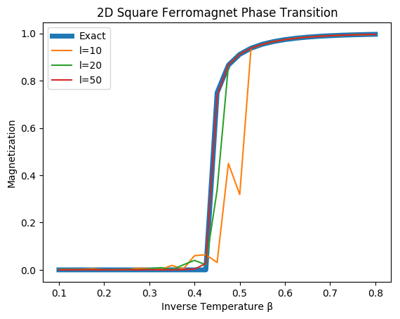
Fig 5: Spontaneous symmetry breaking. As T drops below Tc, the magnetization bifurcates from zero, choosing either a positive or negative macroscopic alignment.
Near the critical temperature , the system exhibits massive fluctuations. The length scale of correlated spins diverges to infinity. Remarkably, the way these systems behave near criticality—defined by their critical exponents—is exactly identical across wildly different physical systems. A boiling fluid and a ferromagnet share the same mathematical exponents. This concept, known as Universality, led to the development of the Renormalization Group, one of the crowning theoretical achievements of the 20th century.